

Hello Friends, in this blog post, we are going to discuss “Excel Data Cleaning” in detail.
Excel is a popular and widely used software application across the world. It greatly helps us in managing…
…sales reports, customer records, employee information, inventory lists, academic results, and financial data.
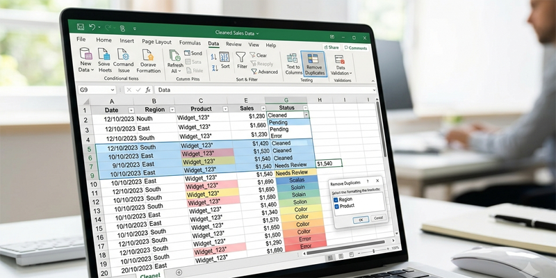
A spreadsheet is only valuable when it contains quality information and is free from inconsistent spellings, duplicate entries,…
…missing values, incorrectly formatted dates, numbers stored as text, and any kind of misleading information affecting reports.
There are several tools provided within Excel to overcome these problems efficiently.
Excel data cleaning greatly helps us improve accuracy; filtering displays the required information, sorting arranges records…
…in a meaningful order, and important patterns can easily be highlighted automatically with conditional formatting.
In this post, we are going to explore “Excel Data Cleaning” in easy-to-understand language.
Here we will learn to clean and organise Excel data, applying filters, identifying errors,…
…highlighting important values, and preparing Excel sheets for reliable or error-free reporting.
What Is Excel Data Cleaning?
Data cleaning is the process of identifying and correcting problems in a dataset so that the information becomes consistent, accurate, and suitable for analysis.
Consider a customer list containing the following entries:
| Customer Name | City | Phone |
|---|---|---|
| Rahul Sharma | Delhi | 9876543210 |
| rahul sharma | Delhi | 9876543210 |
| Priya Verma | Mumbai | 9876501234 |
| Amit Kumar | delhi | 9876512345 |
| Neha Singh | 9876598765 |
This dataset contains several potential issues:
- Rahul Sharma appears twice and may be a duplicate.
- The same city is written as both “Delhi” and “delhi”.
- One customer record has a missing city.
- Phone numbers should be checked for consistency and completeness.
Cleaning the data before analysis can help prevent incorrect customer counts, inaccurate summaries, and unnecessary duplication.
1. Remove Duplicate Records in Excel
Duplicate records can distort sales totals, customer counts, inventory reports, and other calculations. Excel’s Remove Duplicates feature helps remove repeated entries from a selected range.
Steps to remove duplicates
- Select the data range or click inside your Excel Table.
- Open the Data tab.
- Select Remove Duplicates.
- Choose the columns Excel should use to identify duplicates.
- Click OK and review the summary of removed duplicate values.
For example, if a customer list contains the same customer ID multiple times, you might select only the Customer ID column to identify duplicates.
However, if the dataset contains sales transactions, two rows with the same customer name may represent two legitimate purchases. Do not remove records simply because one field matches.
Best practice: Make a copy of the original data before removing duplicates. Always decide what constitutes a genuine duplicate according to the purpose of your dataset.
Identify duplicates without deleting them
You can highlight repeated values using conditional formatting or count occurrences with a formula such as:
=COUNTIF($A$2:$A$100,A2)>1
This returns TRUE when the value in A2 appears more than once in the specified range.
You can use this formula in a helper column or apply a conditional formatting rule to identify repeated entries.
2. Find and Replace Inconsistent Data
The Find and Replace tool helps you locate specific text or values and replace them with a consistent alternative.
For example, a spreadsheet might contain different spellings of a region:
- North
- north
- NORTH
If you want to standardise these entries, select the relevant range, press Ctrl + H, enter the text to find and its replacement, and review the options before choosing Replace or Replace All.
Be careful when replacing short words or numbers. A broad replacement may unintentionally change text inside other values. Select the appropriate range and use whole-cell matching options where suitable.
Find and Replace is useful for:
- Correcting repeated spelling mistakes
- Standardising department names
- Updating outdated category labels
- Replacing unwanted characters
- Correcting consistent formatting errors in imported data
For larger datasets, Power Query can provide a more repeatable approach to standardisation and transformation.
3. Clean Extra Spaces with TRIM
Extra spaces can cause problems when matching names, comparing categories, or performing lookup operations.
For example, Excel may treat Delhi and Delhi as different text values when leading or trailing spaces are present.
The TRIM function removes leading and trailing ordinary spaces and reduces repeated ordinary spaces between words to single spaces.
Formula:
=TRIM(A2)
If A2 contains:
Rahul Sharma
The formula returns:
Rahul Sharma
Apply TRIM to an entire column
- Insert a helper column beside the original data.
- Enter
=TRIM(A2)in the first data row. - Copy the formula down.
- Check the cleaned results.
- If appropriate, copy the results and use Paste Special → Values to replace the original data.
TRIM does not remove every possible nonprinting character. If data has been copied from websites or external systems, you may also need CLEAN or additional text-replacement steps.
4. Handle Missing Values and Blank Cells
Missing data is common in imported spreadsheets, survey responses, customer records, and inventory lists.
Blank cells may represent information that was never entered, unavailable information, or a value that genuinely does not apply. Before filling blanks, determine what they mean.
Find blank cells using Go To Special
- Select the relevant range.
- Press Ctrl + G or F5.
- Choose Special.
- Select Blanks.
- Review the selected cells before making changes.
The exact navigation may vary slightly by Excel version.
Ways to handle missing information
- Leave a cell blank if the information is genuinely unknown.
- Enter an agreed label such as “Not Available” when appropriate.
- Use a verified source to complete missing information.
- Exclude incomplete records from a specific analysis only when the exclusion is justified.
- Use a formula to flag missing required values.
For example, if customer names are in A2 and phone numbers are in B2, use:
=IF(OR(A2="",B2=""),"Incomplete","Complete")
This identifies records where either required field is blank.
Do not automatically replace every blank with zero. A zero may be a meaningful numeric value, while a blank often means missing information.
5. Standardise Dates, Numbers, and Text
Inconsistent data formats can create errors in sorting, filtering, formulas, and reports.
Format dates consistently
Select the date column and choose an appropriate date format from the Home → Number Format options.
For example, dates can be displayed as 29-Oct-2026 or 29/10/2026.
Changing the display format does not necessarily convert text that looks like a date into a genuine Excel date value. If dates are stored as text, you may need to convert them using Text to Columns, a suitable formula, or Power Query.
Standardise numbers
Numbers imported from external sources may be stored as text. Signs can include unexpected left alignment, formulas that do not calculate as expected, or warning indicators.
Depending on the data, you can use the Convert to Number option, Text to Columns, or a suitable conversion formula.
For example:
=VALUE(A2)
This attempts to convert recognised numeric text into a number.
Keep identifiers as text when necessary
Phone numbers, postal codes, and product IDs may contain leading zeros. Converting these values into numbers can remove those zeros.
For example, a postal code such as 012345 should generally be preserved as text or handled with an appropriate fixed-width format.
Important: Formatting a cell as Number is not always enough to repair incorrectly imported data. Check the underlying value as well as its appearance.
6. Sort Data in Excel
Sorting arranges information into a chosen order. You can sort alphabetically, numerically, chronologically, or according to a custom sequence.
Sort one column
- Click a cell inside the dataset.
- Open the Data tab.
- Choose Sort A to Z or Sort Z to A, or select the appropriate ascending or descending option for your data.
For a date column, ascending order places earlier dates before later dates. For a numeric column, ascending order places smaller numbers before larger numbers.
Sort by multiple columns
Suppose you have a list of employees with columns for Department, Name, and Salary.
You can sort first by Department and then by Salary.
- Select the dataset.
- Choose Data → Sort.
- Select Department as the first sorting level.
- Add another level for Salary.
- Choose the desired order for each level.
- Click OK.
Excel groups employees by department and then sorts them by salary within each department.
Use custom sorting
Custom sorting is useful when the desired order is not alphabetical.
For example, you may want priority levels in this order:
- High
- Medium
- Low
Depending on your Excel version, you can create or select a custom list in the Sort dialog.
Best practice: Sort the complete dataset, not just one column. Sorting an individual column independently can separate values from their corresponding records and corrupt the data.
7. Filter Data to Display Relevant Records
Filtering temporarily hides records that do not match your chosen conditions. Unlike deleting rows, filtering does not normally remove the underlying records.
Apply AutoFilter
- Click inside your dataset.
- Select Data → Filter.
- Open the dropdown arrow in the relevant column heading.
- Select the values or conditions you want to display.
For example, if your worksheet contains sales records for several regions, you can filter the Region column to show only North.
Filter by text
Text filters can help you display records that:
- Begin with a particular word
- Contain specific characters
- Match a chosen value
- Do not contain a particular term
For example, you can filter a product list to display names containing “Laptop”.
Filter by numbers
Number filters allow you to show values that meet conditions such as:
- Greater than 10,000
- Less than 5,000
- Between two values
- Equal to a specific amount
- Among the top or bottom items
Filter by dates
Date filters can display records from a particular month, quarter, year, or date range, provided Excel recognises the values as dates.
Filtering is useful when you need to review selected records without changing the entire worksheet.
8. Use Advanced Filters for More Complex Conditions
Excel’s Advanced Filter feature can extract records that meet more specialised criteria.
For example, you may want to display sales records where the region is North and sales exceed ₹20,000.
Create a criteria range with matching column headings:
| Region | Sales |
|---|---|
| North | >20000 |
Then select the source data and open Data → Advanced in supported Excel versions.
Choose the list range and criteria range, and decide whether to filter the data in place or copy the matching records to another location.
When multiple criteria are placed on the same criteria row, they are generally treated as AND conditions. Criteria on separate rows can represent OR conditions.
Advanced Filter is useful for extracting selected records or unique records without repeatedly changing the ordinary filter settings.
9. Conditional Formatting: Highlight Important Data Automatically
Conditional formatting changes a cell’s appearance when it meets a specified condition. It helps users spot important values, trends, and exceptions quickly.
Highlight cells based on values
Suppose you have sales figures in B2 and want to highlight sales above ₹20,000.
- Select B2.
- Open Home → Conditional Formatting.
- Choose Highlight Cells Rules → Greater Than.
- Enter
20000. - Select a formatting style and confirm.
Excel highlights cells that satisfy the rule.
You can similarly highlight values below a threshold, text containing a particular word, duplicate values, or dates within a chosen period.
Use colour scales
Colour scales assign different colours to values across a range. They can help you identify high, medium, and low values quickly.
For example, a sales report might use a colour scale to show the relative performance of different branches.
However, colour scales communicate relative differences within the selected range. They do not necessarily indicate whether a value meets a business target.
Use data bars
Data bars display horizontal bars inside cells, with longer bars generally representing larger values.
They are useful for comparing sales, expenses, marks, or inventory quantities without creating a separate chart.
Use icon sets
Icon sets can display arrows, traffic-light symbols, or other indicators according to specified thresholds.
For example, a performance report could use icons to distinguish high, medium, and low performance.
Check the rule thresholds to ensure the icons communicate the intended meaning.
10. Create Formula-Based Conditional Formatting Rules
Formula-based conditional formatting lets you highlight cells or entire rows according to custom logic.
Suppose your worksheet contains:
- Column A: Product
- Column B: Sales
- Column C: Target
To highlight sales values that are below their corresponding targets, select B2 and create a new conditional formatting rule using:
=B2<C2
Excel evaluates the formula for each selected row. If the condition is true, the selected cell receives the chosen formatting.
Highlight an entire row
Suppose your data occupies A2 and you want to highlight the entire row when the status in column E is “Pending”.
- Select A2.
- Open Home → Conditional Formatting → New Rule.
- Choose the option to use a formula to determine which cells to format.
- Enter:
=$E2="Pending"
- Choose a formatting style and confirm.
The dollar sign before E locks the status column, while the row number changes for each record.
This technique is useful for highlighting overdue tasks, pending orders, low-stock products, and employees who need attention.
11. Use Conditional Formatting to Identify Duplicates
Duplicate entries can be highlighted without deleting them.
- Select the column or range you want to check.
- Open Home → Conditional Formatting.
- Choose Highlight Cells Rules → Duplicate Values.
- Select a formatting style and confirm.
Excel highlights repeated values within the selected range.
For more control, use a formula such as:
=COUNTIF($A$2:$A$100,A2)>1
Apply it to the relevant range through a formula-based conditional formatting rule.
This approach can help identify duplicate invoice numbers, customer IDs, product codes, and email addresses.
Be careful when checking entire rows: two records with the same name may be legitimate separate transactions. Decide which combination of fields defines a duplicate before removing anything.
12. Combine Sorting, Filtering, and Conditional Formatting
These features become more useful when combined.
Imagine a sales worksheet containing product names, regions, sales values, targets, and order statuses.
You can:
- Clean the source data and remove confirmed duplicate records.
- Sort the records by region and sales amount.
- Filter the worksheet to show a particular region.
- Apply conditional formatting to highlight sales below target.
- Use formula-based rules to flag pending orders.
- Create a summary table or PivotTable for reporting.
This workflow allows you to find underperforming products, review incomplete transactions, compare regional results, and prepare reports more efficiently.
For a repeatable monthly process, consider converting the source range into an Excel Table. This can make filtering and expanding the dataset easier.
13. Common Mistakes to Avoid
Removing duplicates without checking the business meaning
Repeated customer names or product names do not always represent duplicate records. Check unique identifiers or the relevant combination of fields.
Sorting only one column
Sorting a single column separately can break the relationship between values in a record. Sort the complete table or a properly selected range.
Treating text numbers as numeric values
Numbers stored as text may not sort or calculate as expected. Check and convert the data where appropriate.
Applying conditional formatting to the wrong range
Formula-based rules depend on the selected range and relative cell references. Test the rule on a few rows before applying it to a large dataset.
Overusing colours
Too many colours and icons can make a worksheet harder to understand. Choose consistent formatting and reserve strong visual emphasis for important information.
Forgetting to check hidden records
Filters can hide rows without deleting them. Before preparing totals or sharing a worksheet, verify that the displayed records and calculations represent what you intend to report.
Frequently Asked Questions
1. What is the difference between sorting and filtering in Excel?
Sorting rearranges records into a selected order, while filtering hides records that do not meet your chosen criteria. Sorting changes the order of the displayed data; filtering changes which records are visible.
2. Does removing duplicates delete the original data permanently?
Remove Duplicates deletes repeated records from the selected range. It is best to create a backup before using it, especially when the data is important or the duplicate criteria are uncertain.
3. Can conditional formatting update automatically?
Yes. Excel generally reevaluates conditional formatting rules when relevant cell values change, subject to calculation settings and the rule configuration.
4. How can I highlight an entire row based on one cell?
Select the full data range and create a formula-based conditional formatting rule. For example, =$E2="Pending" highlights rows where column E contains “Pending”, assuming the selection begins at row 2.
5. Which Excel feature is best for cleaning large datasets?
Excel’s built-in tools are useful for common cleaning tasks. For larger datasets or processes that must be repeated regularly, Power Query is often a better option because it can record transformation steps and repeat them when data is refreshed.
Conclusion
Friends, in this post, we have fully understood the concept of “Excel Data Cleaning“. For maintaining reliable spreadsheets, data cleaning, sorting, filtering, and conditional formatting are some essential Excel skills. Cleaning brings data consistency, sorting organises records better, filtering helps in finding the relevant information, and conditional formatting helps in identifying important values and exceptions easily.
Always try to start with a fresh and clean dataset(Excel Data Cleaning), check for duplicate entries, use standard formats, and resolve missing information. Then, to highlight the important information that actually matters most, wisely use the features of sorting and filtering to explore the records and conditional formatting.
Using these extensive Excel features(Excel Data Cleaning), you can surely make your Excel spreadsheets more accurate, readable, and useful for daily tasks, business analysis, and professional reporting.
If you have any questions, write to us at support@a5theory.com; we will get back to you ASAP.
Hope! You will have enjoyed this post, “Excel Data Cleaning“.
Please feel free to share your feedback in the comments below.
Have a great time!